A little bit about back-propagation.

Or nudging weights in the right direction.

How do neural networks actually work? We have millions of weights and so on, some training data, but how do we go about adjusting those weights to match the training data?

Let’s find out by exploring an extremely simple example to illustrate the core principles.

A single neuron

Let’s create a really simple neural network! We’ll try and get the neural network to learn the OR function. OR is 1 when any argument is 1, and 0 when both arguments are zero. It takes an input X with two elements (either 0 or 1) and outputs y.

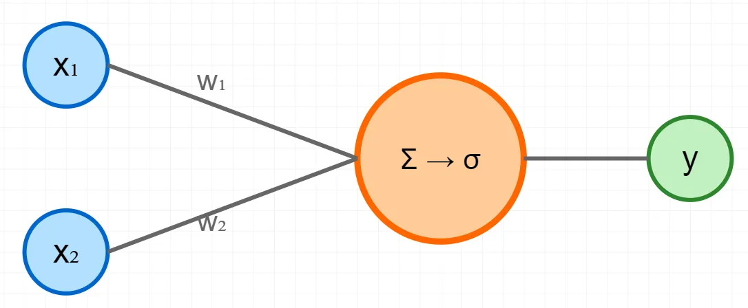
The middle bit is the neuron. And its output is given by the following bit of maths.

\(\begin{align*} y&=\sigma(w_1x_1+w_2x_2) \\ \sigma(z)&=\frac{1}{(1+e^{-z})} \end{align*}\)

σ is an activation function. What’s the point of an activation function? Well, it serves several purposes. Without non-linearity, no matter how many layers you stack, your network could only ever compute linear functions - basically fancy linear regression, not the complex patterns neural nets are famous for learning.

This is such a small example that we can try and work out what the weights “should” be. Let’s start with the values 0 and 0. Since we’re doing the OR function, we want the value of that to be zero.

\(\begin{align*} y&=\sigma(w_1 \times 0 + w_2 \times 0) \\ y &= \sigma(0) \\ y &= 0.5 \end{align*}\)

And you can see that we’re already in trouble! There are no possible weight values the neuron can learn that’ll get the right answer. We fix this, by adding a bias term. Think of this as another learnable parameter for the neuron (alongside w1 and w2). Or more simply, the bias term allows the neuron to output a non-zero value even when all inputs are zero.

\(y=\sigma(w_1x_1+w_2x_2+b)\)

What does that look like in code? It’s a handful of lines of C# (or any other language I hope!) code.

private double _w1 = 0;
private double _w2 = 0;
private double _bias = 0;

public double FeedForward(double x1, double x2) => 
    Sigmoid(_w1*x1 + _w2*x2 + _bias); 

private double Sigmoid(double x) =>
    1.0 / (1.0 + Math.Exp(-x));

Let’s initialize our weights to some starting values ([-4.0 -4.0]) and we’ll start the bias at 0 too and see how we do for the example [1 0]. I’ll spell things out explicitly for my benefit!

\( \begin{align*} y & =\sigma((-4 \times 1) + (-4 \times 0) + 0)\\ y& =\sigma(-4) \\ y&=\frac {1} {1+e^{4}} \\ y&=0.18ish \end{align*} \)

So, with the weights we’ve “randomly” picked we think 1 OR 0 is nearly 0. That sucks! We know the answer, it’s 1. That’s an absolute error of nearly 1! It’s almost exactly wrong.

The good thing with a small example is that we can visualize the whole “loss landscape”. Since visualizing four dimensions isn’t feasible, we’ll simplify the problem by fixing the bias to zero. We’ll take the mean squared error (the difference between what our network predicted and the actual value squared) and plot out our function above for various weight values.

The loss landscape.

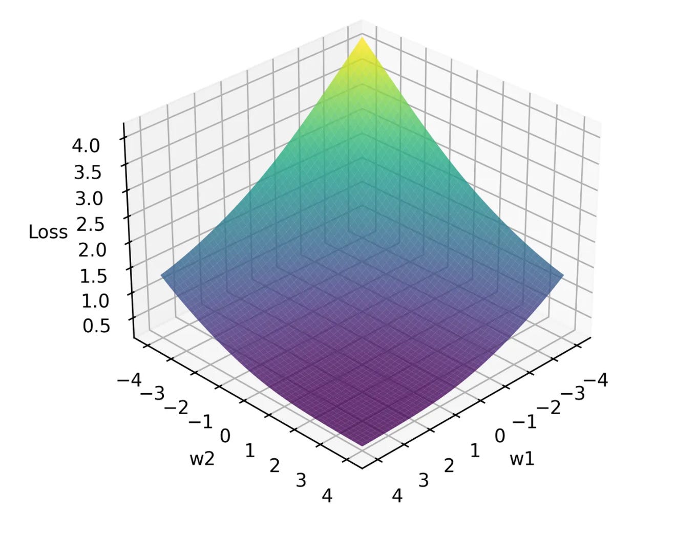
In a strange coincidence (almost as if those random weights weren’t random). It turns out we’re standing at the top of the loss function hill. We know our target too, it’s where the gradient is zero. How should we update our weights?

Updating Weights

The activation function has a nice property that its derivative is very simple to calculate:

\(\begin{align*} \sigma(z)&=\frac{1}{(1+e^{-z})} \\ \frac{d\sigma(z)}{dz} &= \sigma(z)(1-\sigma(z)) \end{align*}\)

So now we can calculate the derivative at any point. In the surface data above, this derivative basically gives us the direction to the answer. So now we just nudge the weights in the right direction and repeat the process. Here’s the code.

public void Backpropagate(
  double x1, 
  double x2, 
  double error, 
  double learningRate)
{
  double output = FeedForward(x1, x2);
  double sigmoidDeriv = SigmoidDerivative(output);
      
  _w1 += learningRate * error * sigmoidDeriv * x1;
  _w2 += learningRate * error * sigmoidDeriv * x2;
  _bias += learningRate * error * sigmoidDeriv; 
}

You’ll notice a new parameter, learningRate, has been introduced. This controls how far we step in each direction. Remember we only know the slope we are standing on - move too far in the wrong direction and we might overshoot the valley.

Imagine a more complicated loss landscape like the below. You’re aiming for the black hole in the middle where the loss is zero. If your learning rate is too high, then you’re going to keep stepping back and forth over minimum. Equally, if your learning rate is too low, then you’re going to tentatively move tiny amounts and never make it.

A more complicated loss landscape (and a nice picture)

So now we’ve got forward and backward. We can run the network forward and work out a prediction given some input. And we can run backwards (backward propagation) and adjust those weights, so they are closer to the target.

Put this all together, and we can now run our training loop.

  double[][] inputs        = {[0, 0], [0, 1], [1, 0], [1, 1]  };
  double[] expectedOutputs = [ 0,      1 ,     1,      1 ]; 

  for (int epoch = 0; epoch < epochs; epoch++)
  {
      double totalError = 0;     
      for (int i = 0; i < inputs.Length; i++)
      {
          double output = neuron.FeedForward(inputs[i][0], inputs[i][1]);
          double error = expectedOutputs[i] - output;               
          neuron.Backpropagate(
            inputs[i][0], 
            inputs[i][1], 
            error, 
            learningRate);
      }
  }

And lo and behold, with a bit of training, it works!

Input: [0, 0], Output: 0.080855, Expected: 0
Input: [0, 1], Output: 0.950012, Expected: 1
Input: [1, 0], Output: 0.949906, Expected: 1
Input: [1, 1], Output: 0.999756, Expected: 1

Being a bit more sophisticated

So, that’s backpropagation (in the simplest way I could think of!).

In the code above, we used a fixed learning rate. That means we’ve got to pick a number and fix it for the whole time. This can be very slow to optimize, because we’ve got to take the same size step regardless of the distance we travel.

Adam (short for Adaptive Moment Estimate) is a technique to address those limitations and it means if you’re training a large model you can make faster progress to minimizing your loss. For each learnable parameter (weights and bias), it adds a couple of different ideas:

1. Momentum - Think of this as strength of direction. If the ball is rolling down the hill, then momentum will keep us going in that direction

2. Adaptive learning rates - If the weight has been changing a lot, then chances are we’re in an undulating landscape so we should slow down. Equally if a weight has barely changed, let’s make bigger steps!

What does this look like? Surprisingly simple! In the code below, AdamParameter is just a class with properties for Value, Momentum and Velocity. beta1 , beta2 and epsilon are just constants values from the paper initialized to sensible defaults, and timeStep just records how far we are along in the process.

  public void Backpropagate(
      double x1, 
      double x2, 
      double error, 
      double learningRate)
  {
      timeStep++;
      
      double output = FeedForward(x1, x2);
      double sigmoidDeriv = SigmoidDerivative(output);
      
      double gradientW1 = error * sigmoidDeriv * x1;
      double gradientW2 = error * sigmoidDeriv * x2;
      double gradientBias = error * sigmoidDeriv;
      
      // Update Adam state for each parameter
      UpdateAdamParameter(_w1, gradientW1, learningRate);
      UpdateAdamParameter(_w2, gradientW2, learningRate);
      UpdateAdamParameter(_bias, gradientBias, learningRate);
  }
      
  private void UpdateAdamParameter(
      AdamParameter param, 
      double gradient, 
      double learningRate)
  {
      param.Momentum = beta1 * param.Momentum + (1 - beta1) * gradient;
      param.Velocity = beta2 * param.Velocity + (1 - beta2) * gradient * gradient;
      double momentumCorrected = param.Momentum / (1 - Math.Pow(beta1, timeStep));
      double velocityCorrected = param.Velocity / (1 - Math.Pow(beta2, timeStep));
      param.Value += learningRate * momentumCorrected / (Math.Sqrt(velocityCorrected) + epsilon);
  }    

The end result is that Adam often converges much faster than the standard gradient descent, and this means lower error rates in fewer iterations.

Why doesn’t it get stuck?

You might be thinking there are some edge cases. If you just consider a 3D surface and finding the lowest point you can easily imagine edge cases where training would fail to converge. You could create a “flat spot” (also known as a saddle point) so that the gradient is zero and weights don’t get updated. Or you could create some deep wells that gradient descent could fall into and never get out.

An unpleasant loss landscape.

In extremely high-dimensional spaces (like our 10 billion parameter network), the statistical likelihood of all dimensions creating a perfect trap becomes vanishingly small. It's a bit like trying to balance a pencil perfectly on its tip - theoretically possible, but practically, any tiny disturbance will cause it to fall in some direction.

Flat regions(where the gradients are close to zero) do exist in high-dimensional spaces. Techniques like the Adam optimizer help, by increasing momentum and velocity so that these areas can be travelled over rather than get stuck.

Conclusion

So that’s back-propagation. Adjust the weights based on the error by calculating the gradient and heading in the right direction. You can get a bit smarter by dynamically adjusting how far you jump.

This simple mechanism (albeit scaled up to a huge number of parameters) is what powers everything from ChatGPT to image recognition systems.