Four Things Queueing Theory can teach us about software development

Software Development is a Game of Queues

Developing software is a game of queues. From a backlog of user stories to be picked up, to a PR awaiting review, to waiting for a deployment pipeline to run on limited infrastructure, our work is fundamentally shaped by queues.

But how often do we step back and think about the mathematics that governs these queues? Queueing theory might sound like an abstract mathematical concept far removed from your daily work, but its principles quietly dictate the rhythm of software delivery in ways that might surprise you.

In this post, I'll explore four counter-intuitive lessons from queueing theory that can transform how you think about software development processes. Whether you're a developer wondering why that "quick fix" is taking forever to reach production, a team lead struggling with sprint planning, or an engineering manager trying to improve delivery predictability, these insights might just challenge some of your core assumptions about productivity and efficiency.

Let's dive into the fascinating world of λ, μ, and ρ - and discover some counter-intuitive truths that might help you deliver more value!

Queueing Theory

Queuing theory examines how systems with limited resources handle incoming requests. The key parameters are:

• Arrival rate (λ): How frequently things enter the queue

• Service rate (μ): How many things can be processed per time unit

The arrival rate is typically modelled as a Poisson distribution. The Poisson distribution predicts how many times an independent random event will occur within a fixed period. For this model to be applicable, the things arriving in the queue are independent, randomly distributed and the average arrival rate is known.

The service rate is typically modelled as an exponential distribution. Service times aren’t constant (we’ve all experienced being behind that person in the supermarket who has vouchers a plenty and a life story to tell).

Putting all this together, we can model a queue with a given arrival rate and service rate with a single person doing some work. This is known as an M/M/1 queue (see Kendall’s notation) and is the simplest one to model! Here’s some code.

Let’s assume an average arrival rate of 4 per minute, and an average 5 customers served per minute and simulate it for 500 units. You might expect that the queue stays fairly constant, but it doesn’t. Sometimes, you get people bunched up. Sometimes you get work taking longer. And you end up with large queues.

Queue Length over time (arrival=4, service=5).

And as well as large queues, you also can end up with zero queues. This is known as utilization (ρ) and is the ratio of arrival rate to service rate (λ/μ). In this example, we’re running at a utilization rate of 80% (4 divided by 5). What happens if we ask folks to work harder?

100% Utilization is not the goal.

A utilization rate of 80%? Clearly that’s waste. 20% of their time those pesky workers are sitting on their bottoms twiddling their thumbs. Obviously, we should aim for 100% utilization!

Let’s tweak the parameters and set the arrival rate and service rate to be the same (5) and re-run our simulation and see what happens.

Queue Length over time (arrival=5, service=5)

Oh dear. Our queue length is now huge. And if we plot out the wait times, we see that most people are waiting for over 5 units of time (it’s less than 1 in the previous example).

Histogram of waiting times

It turns out that the closer utilization is to 1, the longer the average waiting time. In fact, wait times approach infinity as utilization approaches 100%.

As utilization increases, the average rating time goes to infinity

Limit Work in Progress

Little’s Law is a fundamental principle in queueing theory that establishes the relationship between throughput, lead time and work in progress. It’s a nice simple formula! The formula says that the average number of work in progress items is equal to the arrival rate multiple by the average time in the system (W).

\(L=\lambda W\)

We can already see this in our examples above. In the second example, the average wait time is five, multiple that by the arrival rate of four and you get an average of 20 items in the queue at any one time, and that’s (more or less) what the graph shows. We can also rearrange this formula. If we constrain WIP and the throughput remains constant, then the average time in the system must decrease.

\(W=L/\lambda\)

Let’s use the same example above, to try and deliberately limit work in progress (WIP) and see what happens. We keep the arrival time and service rate same as before (4 and 5 respectively) and just turn items away (ignore them completely) if the queue gets longer than 5.

Wait times are higher without a WIP limit

So, the good news is that implementing a WIP limit worked - throughput has improved with the average time things wait in the queue dropped from 0.65 to 0.36. Nice!

Of course, the WIP limit means that some items are discarded and not put in the queue. You might think that’s bad? But remember, most features you write will go unloved or unused. Would you rather say “no” a few ideas in exchange for faster throughput? Seems like a good trade to me.

If you want to improve throughput, limit work in progress.

Don’t batch work up!

Let’s now, connect three queues together and imagine they represent Development, Test and Deployment. We’ll treat each of these queues as M/M/1 queues (as above) and we’ll compare two options.

1. Single piece flow - Each job starts as soon as possible

2. Batch mode - we’ll group things into chunks of five and not start work until the last item in the batch arrives.

When you write things down like this, it’s kind of obvious that batch mode is slower. We’ve got two sources of delay with batch mode - firstly waiting for the batch to fill, and then secondly the processing of it.

We can see it with the simulation (arrival rate 4, service rate 5 for all stages).

Batching work up keeps work in the system for longer

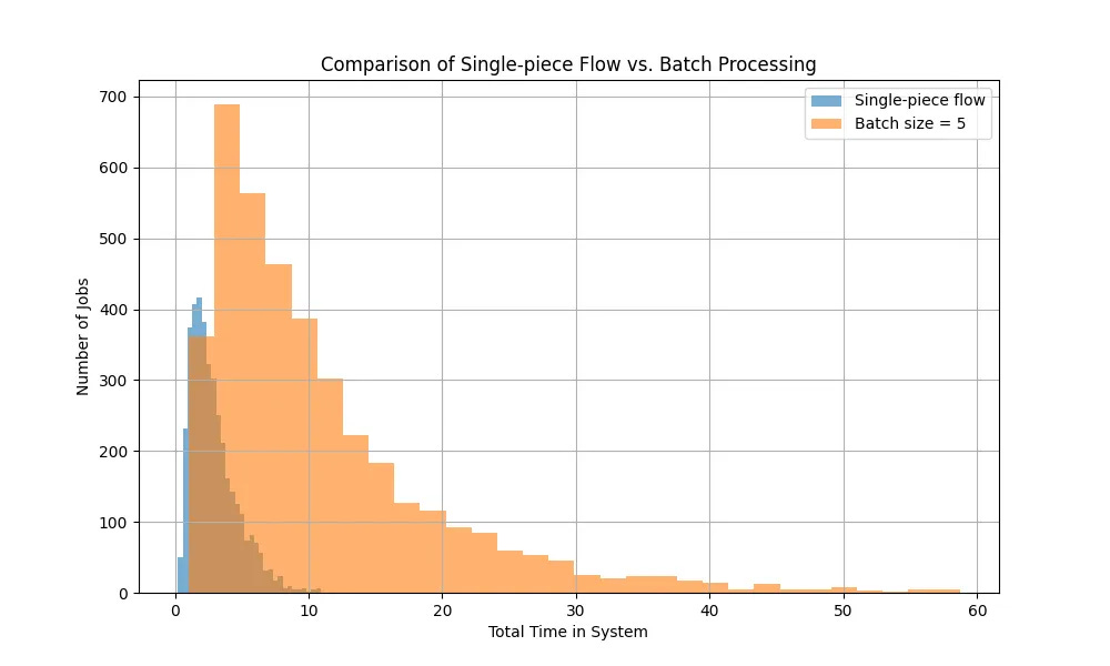
Well, that indicates what is obvious. So why would anyone batch up work and do big releases? I guess there’s an assumption that batching things up could result in some efficiency gain. Perhaps running the test workflow is more efficient because I can test five things quicker than one at a time? For example, perhaps it requires a length set up procedure.

How much faster would you have to be in “batch mode” to reach that distribution for single piece flow? The honest answer is that it wouldn’t help. The problem is that the batching delay itself (waiting for those features) dominates. For example, when you’re batching you can be stuck waiting for a batch for fill (those random arrival times really add up!).

What does this mean for software development? Aim for single piece flow.

Only focus on the bottleneck!

The Goal is a business story by Eliyahu Goldratt that introduces the Theory of Constraints (TOC). The key insight of this approach is that a systems throughput is limited by its most constrained component. Improving anything other than the bottleneck is an illusion.

Why is this? Improving upstream processes leads to more queues at the bottleneck. Downstream of the bottleneck enhancements remain underutilized because the arrival rate into those queues is constrained by the bottleneck.

We can see this by sticking some M/M/1 queues together with different processing rates. The first and last stages are fast, and the middle stage (stage 2) is the bottleneck with a slower processing rate. Stage 1 and 3 have the same processing rate (6 per time period) whereas Stage 2 is the bottleneck with a processing rate of 5 units per time period.

Improvements other than at the bottleneck are an illusion (mostly)

Improving stage 1 or stage 3 from the original 6 to 10 (a huge increase in performance) makes almost no difference to the baseline performance. Why? Because the performance of the poorest queue dominates! In comparison, nudging the performance of the bottleneck at all has a huge improvement.

What does this mean for Software Development? Find the slowest bit in your pipeline; make it faster. Repeat.

Conclusion

If you want smoother software delivery, and shorter wait times, remember these four takeaways from queueing theory.

• Avoid aiming for 100% utilization to prevent exponential wait times

• Limit work in progress to improve throughput

• Favour single piece flow over batching to reduce delays

• Focus your improvement efforts exclusively on bottlenecks

Applying these insights will help work flow through your system, with less stress and (hopefully) more value delivered!